41 excel pivot table 2 row labels

How to Use Excel Pivot Table Label Filters - Contextures Excel Tips Right-click a cell in the pivot table, and click PivotTable Options. In the PivotTable Options dialog box, click the Totals & Filters tab. In the Filters section, add a check mark to 'Allow multiple filters per field.'. Click the OK button, to apply the setting and close the dialog box. Pivot Table Row Labels In the Same Line - Beat Excel! First make a pivot table with required fields. Arrange the fields as shown in left picture. Your initial table will look like right picture. Now click on "Error Code" and access field settings. First check "None" option in "Subtotals & Filters" tab to disable totals after every row.

Excel, Pivot and multiple row labels - Super User where "Server" and "Version" are always the same in a row. I would like a pivot table with | Server | Version | DBs | | a | v1 | 3 | | b | v2 | 2 | with DBs as the number of DBs on the given server. Now I only manage to have one column "Server" as Row label. If I add the "Version" column to the list of columns I get something like

Excel pivot table 2 row labels

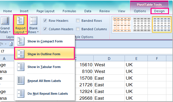
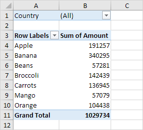
Multi-level Pivot Table in Excel (In Easy Steps) - Excel Easy First, insert a pivot table. Next, drag the following fields to the different areas. 1. Country field to the Rows area. 2. Amount field to the Values area (2x). Note: if you drag the Amount field to the Values area for the second time, Excel also populates the Columns area. Pivot table: 3. Next, click any cell inside the Sum of Amount2 column. 4. Repeat item labels in a PivotTable - support.microsoft.com Right-click the row or column label you want to repeat, and click Field Settings. Click the Layout & Print tab, and check the Repeat item labels box. Make sure Show item labels in tabular form is selected. Notes: When you edit any of the repeated labels, the changes you make are applied to all other cells with the same label. Pivot Table Row Labels - Microsoft Community If you go to PivotTable Tools > Analyze > Layout > Report Layout > Show in Tabular Form, your column headers will be used for the row labels. Every once in a while there's a sudden gust of gravity... Report abuse 1 person found this reply helpful · Was this reply helpful? Yes No A. User Replied on December 19, 2017

Excel pivot table 2 row labels. How to make row labels on same line in pivot table? - ExtendOffice 1. Click any one cell in the pivot table, and right click to choose PivotTable Options, see screenshot: 2. In the PivotTable Options dialog box, click the Display tab, and then check Classic PivotTable layout (enables... 3. Then click OK to close this dialog, and you will get the following pivot ... How to filter a pivot table with multiple filters - Exceljet To enable multiple filters per field, we need to change a setting in the pivot table options. Right-click in the pivot table and select PivotTable Options from the menu. then navigate to the Totals & Filters tab. There, under Filters, enable "allow multiple filters per field". Automatic Row And Column Pivot Table Labels - How To Excel At Excel Select the data set you want to use for your table The first thing to do is put your cursor somewhere in your data list Select the Insert Tab Hit Pivot Table icon Next select Pivot Table option Select a table or range option Select to put your Table on a New Worksheet or on the current one, for this tutorial select the first option Click Ok Formula1, Formula2 appearing as row items in pivot table where row ... Formula1, Formula2 appearing as row items in pivot table where row labels previously were A table than previously showed date, time, address and hours , was now replaced by date, time, formula1, formula2....formula7 as the values in a column and then the duration.

How to Customize Your Excel Pivot Chart Data Labels - dummies The Data Labels command on the Design tab's Add Chart Element menu in Excel allows you to label data markers with values from your pivot table. When you click the command button, Excel displays a menu with commands corresponding to locations for the data labels: None, Center, Left, Right, Above, and Below. None signifies that no data labels ... Data Labels in Excel Pivot Chart (Detailed Analysis) 7 Suitable Examples with Data Labels in Excel Pivot Chart Considering All Factors 1. Adding Data Labels in Pivot Chart 2. Set Cell Values as Data Labels 3. Showing Percentages as Data Labels 4. Changing Appearance of Pivot Chart Labels 5. Changing Background of Data Labels 6. Dynamic Pivot Chart Data Labels with Slicers 7. Excel Pivot Table Row labels - Stack Overflow Right click on the pivot, go to PivotTable Options, Display Tab. Click on "Classic Pivot Table Layout" Go to each field (column), right click, field settings, layout & print tab. Click on "Repeat Item Labels" That should give you the table you're looking for. Share answered Nov 9, 2015 at 13:20 user1923975 1,359 4 13 28 Add a comment Pivot table row labels in separate columns • AuditExcel.co.za So when you click in the Pivot Table and click on the DESIGN tab one of the options is the Report Layout. Click on this and change it to Tabular form. Your pivot table report will now look like the bottom picture and will be easier to use in other areas of the spreadsheet and in our opinion is also easier to read.

multiple fields as row labels on the same level in pivot table Excel ... multiple fields as row labels on the same level in pivot table Excel 2016 I am using Excel 2016. I have data that lists product models along with relevant data and also production volumes by month. Part of the relevant data are about 5 common part columns with the part # that applies to each model under the appropriate column. get a row label from pivot table - Microsoft Tech Community Creating PivotTable add data to data model by checking Create PivotTable and after that convert it to cube formulas. Now you may take these formulas and convert it to form you need, for example in H3 it could be =CUBEVALUE( "ThisWorkbookDataModel", CUBEMEMBER("ThisWorkbookDataModel", " [Measures]. pivot table how to combine 2 row labels | MrExcel Message Board pivot table how to combine 2 row labels sdsurzh Nov 6, 2013 S sdsurzh Board Regular Joined Sep 27, 2009 Messages 248 Nov 6, 2013 #1 Hi, i am having the pivot table in the below format. my concern is how i can combine both A & AA together the source is from data connection and not from the excel. Duplicating row labels in a Pivot Table - Excel 2011 [SOLVED] So I have a pivot table with two row labels (Zone and Ads) and two value parameters in my pivot table. My issue is I would like the pivot table to make my first row label (zone) duplicate for every (ad - second row label) so I do not have to cut and paste it when I transfer the pivot table information elsewhere.

23 things you should know about Excel pivot tables | Exceljet

Pivot Table Row Labels • AuditExcel.co.za Right click on the Row Labels again - go to Field Settings. Look at Layout and Print. At the moment it is ticked as "show item labels in tabular form" - if I said please show the items labels in "outline form" and say OK you will see how the Pivot Table looks changes. Go back to Layout and Print and say "please display labels from ...

Components | CLEARIFY

How to add side by side rows in excel pivot table - AnswerTabs First, you have to create a pivot table by choosing the rows, columns and values: Created pivot table should look like this: You have to right-click on pivot table and choose the PivotTable options. Then swich to Display tab and turn on Classic PivotTable layout: Now the pivot table should look like this: As a next step, you have to modify the Field settings of the rows: In subtotals section choose None:

abc Microsoft EXCEL 2010 - Pivot table - Izdvajanje elemenata PIVOT CHARTS-a

How to rename group or row labels in Excel PivotTable? - ExtendOffice 1. Click at the PivotTable, then click Analyze tab and go to the Active Field textbox. 2. Now in the Active Field textbox, the active field name is displayed, you can change it in the textbox. You can change other Row Labels name by clicking the relative fields in the PivotTable, then rename it in the Active Field textbox.

Pivot Table Excel 2007 Repeat Row Labels | Elcho Table

Pivot Table "Row Labels" Header Frustration Pivot Table "Row Labels" Header Frustration. Hi Everyone please help I can't change my headers from Row Labels in a Pivot Table. Using Excel 365. Labels:

java - How to set default value for row labels in pivot table using poi - Stack Overflow

Use column labels from an Excel table as the rows in a Pivot Table ... Highlight your current table, including the headers. Then from the Data section of the ribbon, select From Table. Highlight all the columns containing data, but not the Year column, and then select Unpivot Columns. Close the dialog and keep the changes. Excel should place the unpivoted data into a new worksheet, looking something like this:

Pin by Larry Xu on Excel | Pivot table, Excel, Row labels

Excel Pivot Table with nested rows | Basic Excel Tutorial Steps 1. Insert your pivot table. Click Insert Menu, under Tables group choose PivotTable. 2. Once you create your pivot table, add all the fields you need to analyze data. How to add the fields Select the checkbox on each field name you desire in the field section. The selected fields are added to the Row Labels area in the layout section.

Pivot Table In Excel 2007 With Example Ppt | Review Home Decor

Multiple row labels on one row in Pivot table - MrExcel Message Board I figured it out - Right click on your pivot table and choose pivot table options/display. Click on "Classic PivotTable layout" Then click on where it is subtotaling your row label and uncheck the subtotal option. D dudeshane0 New Member Joined Oct 23, 2014 Messages 1 Jan 19, 2015 #6 Gerald Higgins said:

How to repeat row labels for group in pivot table?

How to Use Label Filters for Text in the Pivot Table? To know how to create a Pivot table please Click Here. Step 2: To add a field, Tick the checkbox before the field name in the PivotTable Fields panel. When you select the field name, the selected field name will be inserted into the pivot table. Pro Tip. Row Labels are used to apply a filter to rows that have to be shown in the pivot table.

Why pivot table doesn't sort properly row labels? : excel

Pivot table row labels side by side - Excel Tutorials - OfficeTuts Excel You can copy the following table and paste it into your worksheet as Match Destination Formatting. Now, let's create a pivot table ( Insert >> Tables >> Pivot Table) and check all the values in Pivot Table Fields. Fields should look like this. Right-click inside a pivot table and choose PivotTable Options…. Check data as shown on the image below.

Pivot table row labels side by side – Excel Tutorials

How to Concatenate Values of Pivot Table | Basic Excel Tutorial The Excel table should consist of a list of values. Now click any cell inside your data workbook. At the top menu of your workbook, go to the Insert Tab. Under the Insert Tab ribbon, select Tables at the far top-left corner and choose Pivot Table. A dialog box will appear, and Excel will automatically select the data for you. Next, a Create ...

Excel, Pivot and multiple row labels - Super User

Pivot Table Row Labels - Microsoft Community If you go to PivotTable Tools > Analyze > Layout > Report Layout > Show in Tabular Form, your column headers will be used for the row labels. Every once in a while there's a sudden gust of gravity... Report abuse 1 person found this reply helpful · Was this reply helpful? Yes No A. User Replied on December 19, 2017

How To Create Pivot Table With Multiple Columns In Excel 2010 | Awesome Home

Repeat item labels in a PivotTable - support.microsoft.com Right-click the row or column label you want to repeat, and click Field Settings. Click the Layout & Print tab, and check the Repeat item labels box. Make sure Show item labels in tabular form is selected. Notes: When you edit any of the repeated labels, the changes you make are applied to all other cells with the same label.